In the next of our blogs on Building a Digital Twin within the ArcGIS Platform, we look at how we processed the point cloud data of our offices we collected using a Drone and a Laser scanner.
Missed the early instalments of the series? Check out Part 1, Part 2 and Part 3 first.
Introduction
So, at the end Part 3, we had a whole bunch of full resolution geolocated laser-scanned point clouds for our Leeds (128 point clouds, 352Gb data in total) and London (26, 105Gb) offices, and an exterior drone-derived mesh (115Mb) and point cloud (600Mb) for the Leeds office.
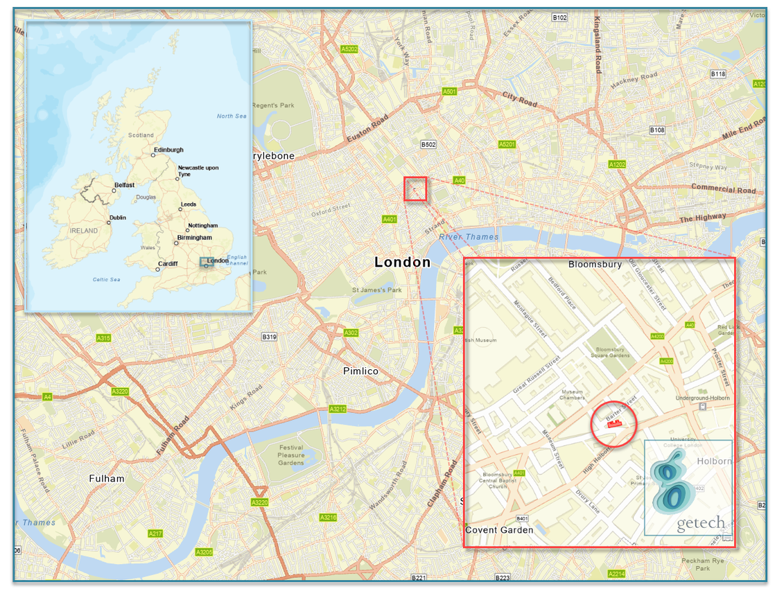
A location map for our London office is provided below to make it easier to understand the later screengrabs, which show our floor of the building floating in mid-air – our office is on the 2nd Floor and we didn’t scan the outside of the building…
LAS format
The point clouds were all in LAS format – which is supported natively by ArcGIS Pro (as is the Esri zLAS compressed format), which is why we’d picked it. It should be noted that the LAS format and the LAS tools within ArcGIS Pro were primarily developed for storing and processing/analysing airborne LiDAR data, not Laser Scanner data. The E57 format has been designed for storing point clouds from Laser Scanners, but is not yet natively supported by ArcGIS Pro. Anyway, back to the story.
Size
We’d published the Drone-derived mesh to ArcGIS Online, and made it available in this out-of-the-box app, which performs well on relatively low-spec hardware (e.g. it works on an iPhone 7). On my laptop, however, the full resolution laser-scanned point clouds are close to being unusable – which is not surprising as each one has c. 160 million points in. The view below took 5 minutes to render on my laptop (you can interact with the view whilst it’s rendering, which makes it far less painful).
So, it was clear we needed to improve the performance and that the obvious way to do that was to cull some of the points, at least temporarily. Fortunately, 3D Analyst provides the Thin LAS tool which allowed us to do exactly that. Thinning the point clouds for our London office to 10 cm (one point in each 10 cm ‘voxel’) reduced the data volume to 22Mb from 105Gb.
Obviously we removed rather a lot of detail there – as you can see if you compare the next screengrab with the last one – but we used the thinned data set for setting up views and operations which we then performed against the full resolution version (or further thinned versions, thinned for specific purposes).
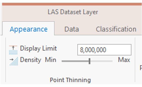
Having thinned the datasets, we then displayed them to see the points, rather than their host datasets’ bounding boxes. Note that I found it helpful to amend the display limit for my LAS layers upwards from the default as that stopped sections rendering and made them disappear.
Unwanted data – noise
The screengrab below shows the 26 thinned LAS files for our London office displayed in a 3D local scene. The red oblong resting on the ground is the footprint of the building, which has been extruded upwards in semi-transparent grey to form the shell of the office building. Either our office has some unusual design features, or we have some issues with our data.
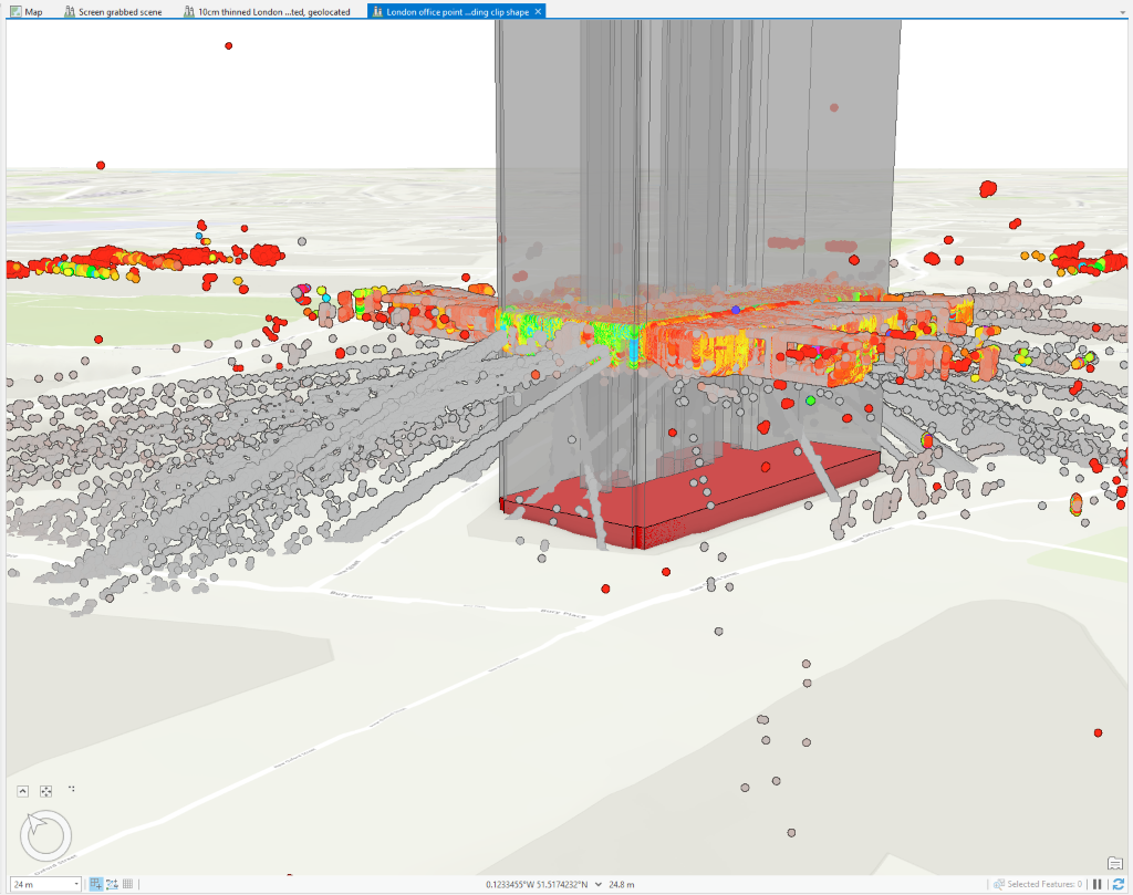
Figure 5 – the unedited, thinned merged point cloud for the London office – note the rooms that apparently protrude far from the building footprint, and what look slides
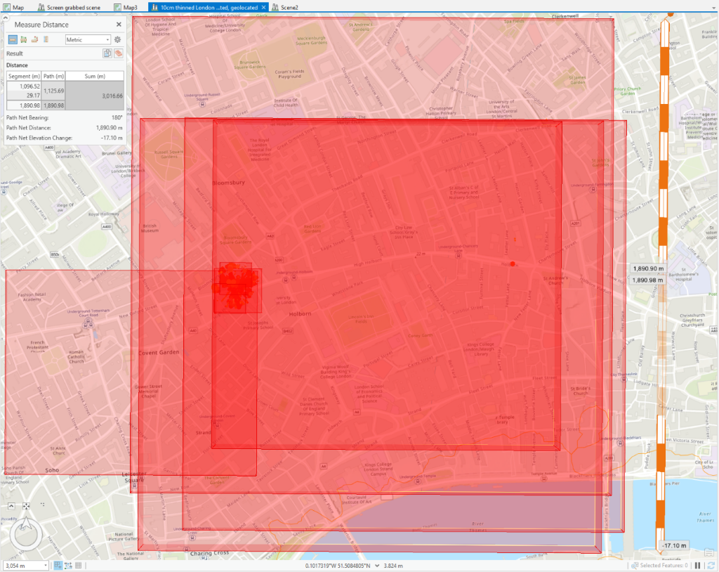
Plotting the bounding boxes of the 26 LAS files, we see that they cover a sizable part of central London.
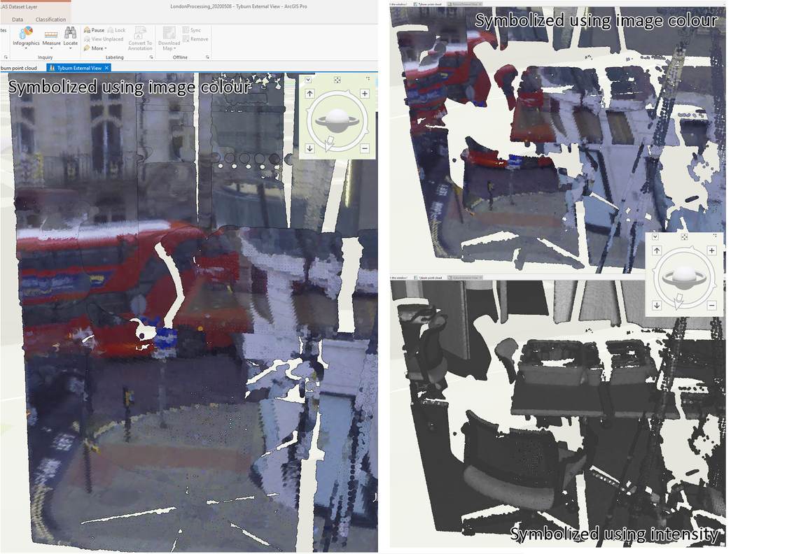
These issues are caused by multiple reflections of the scan beam by exterior and interior windows and the coverings applied to these, as well as reflective light fittings. The screenshots below illustrate how a ‘ghost’ room is created outside the office – the shots on the left are actually taken from the ghost room, looking in.
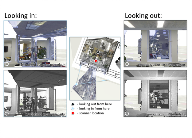
Figure 7 – a ghost room, the central view is top-down on the point cloud, symbolized using image colour
Also illustrated in the screenshots above is the fact that the point cloud colourization (upper images) was done using photographs captured by the instrument, rather than by processing the scan beam returns – those provide an intensity reading (lower images). This methodology has an odd effect here – whilst it looks from the top right image as though we’re looking through the window and seeing the building opposite, we’re actually not – what we’re seeing is the content of the ghost office which has been colourized by the photograph.
Looking out of the window at a different angle (screenshot below, left hand side), we can see a London Routemaster bus – changing the angle slightly splits the bus apart (top right); replacing the colour with the intensity (bottom right) allows us to see that the chair in the foreground of the ghost office has been colourized with the bottom of the bus.
Clipping the data
So, how did we deal with all this unwanted and extraneous data? The answer is that we clipped the LAS files using a building footprint using ArcGIS Pro’s 3D Analyst ExtractLAS tool. This worked well for our London office which has a simple footprint and is all on one floor but had some issues with our Leeds office which has stairs and skylights. The tool only works with 2D (XY) polygons so you can’t extract a 3D volume with it.
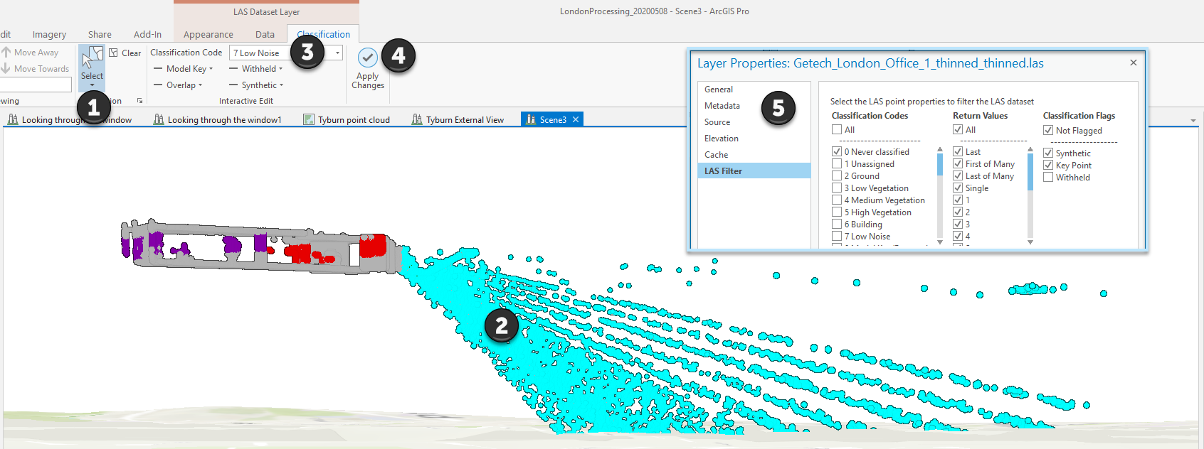
However, there are an array of classification tools, both semi-automated and manual, which allow you to classify LAS points, and you can then hide the classes that you don’t want. If you then use the ExtractLAS tool, the output LAS will not contain the hidden classes. So, you can adopt a two-stage process – stage 1 – extract in the XY planes, stage 2 – classify and remove in the Z plane.
The screenshot above illustrates the workflow:
- Select one of the graphical selection tools on the Classification tab of the LAS Dataset Layer ribbon (having selected a LAS (not zLAS) layer in the table of contents).
- Select a set of points from the LAS.
You may have to do this repeatedly, as I think it only selects the closest point to your viewing position in each direction (try it and you’ll see what I mean). - Select a classification code to apply to the selected points.
The classification codes are pre-defined and aimed at the classification of airborne LiDAR data - Apply the changes.
This saves the classification to the LAS file. - View the properties for the LAS layer and switch off the classes you don’t want to see.
That’s actually a fairly painless workflow, especially considering the tools aren’t aimed at working with this kind of data.
We also, however, implemented a Python tool that uses the LASPY library and allows you to combine an XY clip with a Z extraction and we used this to bulk process all the scans for our London office, giving us a set of scans without ghost rooms and other reflection issues.
Wrapping it up
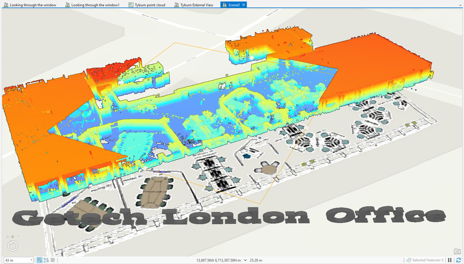
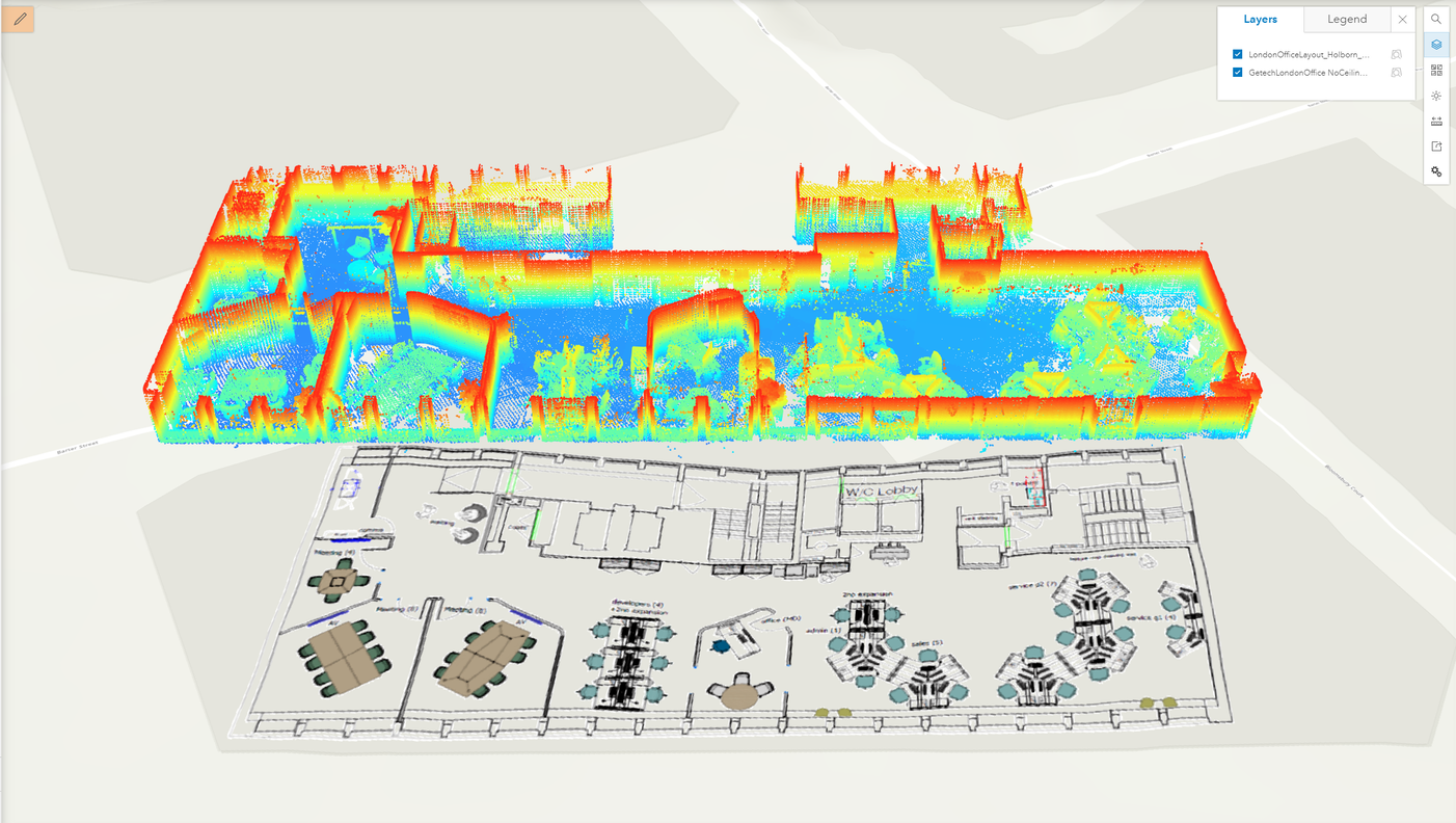
We then merged thinned versions of the scans into a single LAS file that is 17Mb in size, compared with the 105Gb source – it’s thinned to 10cm, so we’ve lost rather a lot of detail, but it’s actually still very usable as a floorplan (see below).
The derived Point Cloud Scene Layer Package (we had to slice the ceiling off so you could see inside on the web) we made with this Pro tool is only 4Mb in size – we’ve published this to our ArcGIS Online, if you’d like to take a look.
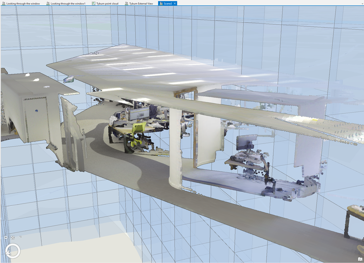
Here’s a screenshot of the merged LAS data in ArcGIS Pro, with a horizontal slice taken out of the ceiling using the 3D Exploratory Analysis Interactive Analysis tool – you can see how the walls and furniture can be easily identified.
In our next blog we’ll look at ways of modelling the features captured by the point cloud to achieve a range of aims, from the creation of a simple floorplan to the capture of the fine detail of ceiling mouldings and wall panels.
Lessons learned:
- Creating and visualizing thinned versions of the data in ArcGIS Pro makes working with the full resolution data easier.
- Make sure you ‘hold onto something’ – if you find yourself zooming through your point cloud and appearing on the other side of it, try putting your mouse on a point or clump of points, as that enables the software to actually know where your mouse is.
- We found that building a 3D grid around our point cloud was a (fairly heavy-handed) way of solving this issue, as illustrated below.
Posted by Ross Smail, Head of Innovation.
