In my last blog post I discussed the case for mapping the residuals in order to help us to understand the quality of the output of the interpolation of a continuous variable.
In there I emphasized the importance of looking at the spatial distribution of the signed residuals to identify whether their spatial distribution may be the result of a random process or a pattern can be identified.
The reason why I am interested in looking at the distribution of residuals is very simple. For the models we have generated by interpolation to be trusted I want their residuals to have two key characteristics:
- To show a spatially random distribution, meaning that no spatial pattern of clusters can be recognised. We want overpredictions and underpredictions to reflect the distribution of a random process as much as possible.
- To be normally distributed, or as close to a normal distribution as possible. This implies that their mean (average) value is, or is close to, zero.
When the two conditions as above are met, I can reasonably trust that my model is unaffected by the presence of bias, i.e. it does not systematically overpredict or underpredict the values of the variable we are modelling.
Using the interpolation algorithms available in Spatial Analyst one can derive the signed residuals from any model generated by interpolation. Do this by using the “Extract Values to Points” tool available in ArcToolbox under ‘Spatial Analyst Tools > Extraction’.
Alternatively, if the Geostatistical Analyst extension is used to generate models, use the “GA Layers to Points” tool in ArcToolbox under ‘Geostatistical Analyst Tools > Working with Geostatistical Layers’. Note that this extension automatically provides the users with an estimation of the quality of the output by means of cross-validation and, in the cases of kriging and cokriging, with maps of error values.
Deriving residuals for my model
An example of residuals for a continuous variable is shown in Figure 1. I have derived these residuals by simply using the point dataset I have used to generate my model and the model itself as input to the “Extract Values to Points” tool. In so doing I have derived, for each location for which my variable has been measured, the corresponding predicted value. I have then added a new field called Residuals to my table and have calculated this field by a simple mathematical operation (Residuals = Predicted – Observed).
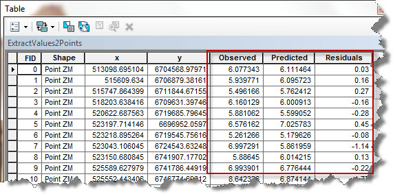
Figure 1: derived signed residuals.
Once I have derived the residuals I can map their signed value. I have simply symbolised the errors based on their sign. In Figure 2 I have used blue dots to highlight underpredictions (negative errors) and red dots to highlight overpredictions (positive errors).
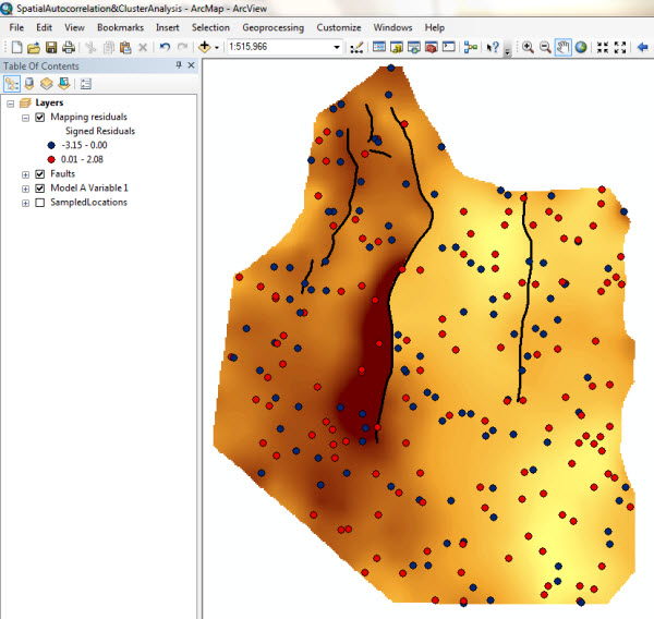
Figure 2: symbolising signed residuals
It is not straightforward to figure out whether a pattern exists in the distribution of the signed errors just by looking at the map. I am therefore in need of a more “robust” approach to carry out the analysis I have in mind.
Using ArcGIS to check residuals bias
ArcGIS provides a number of tools for investigating spatial relationships and assumptions behind spatial modelling. I’m going to focus on a simple tool I can use to gain a quick insight on the spatial distribution of my errors. The tool is called Spatial Correlation (Moran I) and is available in ArcToolbox under ‘Spatial Statistics Tools > Analyzing Patterns’ (Figure 3). Note that this toolbox is available with any level of license and does not require any additional extension to ArcMap.
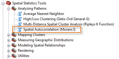
Figure 3: the Spatial Autocorrelation tool in ArcToolbox
The Spatial Autocorrelation computes the degree of heterogeneity among the values of our variable. Local autocorrelation is computed by assigning a weight to neighbouring residuals based on their relative location with respect to each sampled location. In so doing the tool tests whether statistically significant clusters exist in the values of a variable (in my case the values of my model’s residuals).
If that is the case, I’d expect errors to show a pattern in their distribution, and the randomness requirement discussed earlier to not be met, with my model systematically underpredicting or overpredicting values in some particular areas. In these, I would expect my model to seriously misrepresent the reality.
Once I have launched the Spatial Autocorrelation tool in ArcGIS I’ll be asked to specify the layer and variable I want to investigate (see Figure 4).
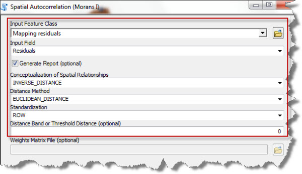
Figure 4: the Spatial Autocorrelation dialog in ArcGIS.
I select the optional “Generate report” box – this generates a summary of the main statistical parameters of the autocorrelation which I’m going to use for my analysis.
Various options are available to describe the variable’s spatial relationship, depending on the type and amount of spatial dependency expected in the data.
Tip: If you are dealing with continuous variables and feel uncomfortable with choosing one choice or the other, use the inverse distance or the inverse distance squared (if you expect the dependency to level off fairly quickly with the distance).
If data has been sampled preferentially and is clustered around some specific areas, I would suggest using the “row” standardisation option, which takes into account the presence of clusters when assigning weights.
I would also specify a cut-off distance if I wanted samples located beyond a certain distance not to be included in the correlation analysis. In my example (Figure 4) I have set the Distance Band option to zero because I did not want a cut-off distance to be used in my analysis.
Making sense of the results
Once I have run the tool, the results are summarised in a report as seen in Figure 5 below. A number of statistical parameters are calculated; among these the ones which are relevant for my analysis are the z-score, p-value and the Moran’s index.
The first two provide an understanding on whether the hypothesis of our residuals to be randomly distributed is statistically valid or not. The z-score measures the spread of the distribution around its mean expressed in standard deviation units. This index tells me whether the population of our residuals is close or far from the ideal normal distribution. Classical statistics tells me that in a normally distributed population 68% of its values fall within plus or minus one standard deviation from the mean and 95% within plus or minus 1.96 standard deviations.
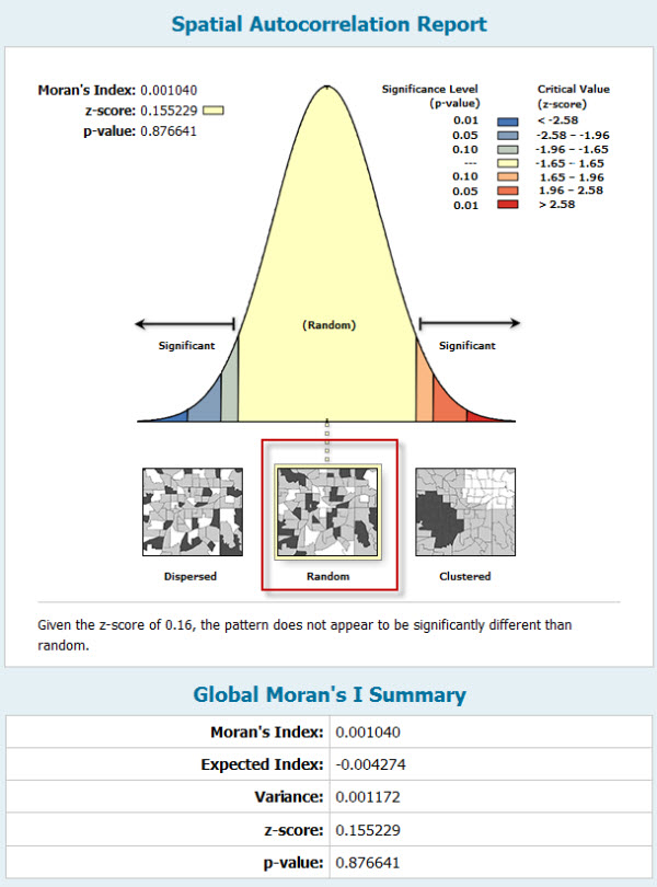
Figure 5: report summarising the results of the spatial autocorrelation analysis
The p-value is a measure of the probability of the distribution being the result of a random process. The p-value is usually considered in comparison with a user-defined level of confidence, often set to 0.05 (confidence level 95%). If my p-value is smaller or equal to the set level of confidence, the likelihood of my residuals to be the result of a random process (for instance when z-score value falls within one standard deviation from the mean) is very low and I would expect residuals to show a pattern in the spatial distribution of their values.
If z-score and p-value indicate that there is the likelihood of a pattern in the spatial distribution of my residuals, the Moran’s Index provides an indication of the nature of this pattern. A positive value indicates a clustered pattern, while a negative value indicates a dispersed pattern. In both cases these patterns cannot be regarded to as the results of a random process.
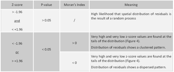
Table 1: summary of spatial autocorrelation resuts
Note that in Table 1 I have assumed two standard deviations from the mean to be a suitable choice for my analysis (z-score cut-off +/- 1.96).
I have also assumed that a level of confidence of 95% is sufficient for the scope of my modelling (p-value cut-off 0.05).
For the example I have used here and the scope of my analysis I would assume that I would be happy with a z-score value within two standard deviations from the mean (+/- 1.96) and a statistical significance of 95% (p-value 0.05).
As shown in Figure 5 my z-score is +0.16 (falls within two standard deviations as I required) and the p-value is 0.88 (higher than the significant value’s threshold of 0.05). In this case I can be quite confident that the distribution of my residuals indicates a random process. I don’t even need to consider the value of the Moran’s Index, as no significant patterns (clustered or dispersed) can be identified.
If, on the other hand, the result of my analysis had shown z-score values falling outside the desired significance and p-values smaller than the required statistical significance, I would have expected a pattern to be identified in the distribution of my residuals. In such a case the sign of the Moran’s Index would have identified whether the pattern would have been a clustered or dispersed one.
In this last case I would probably need to reconsider my modelling process, by choosing a different algorithm or changing the parameters controlling the interpolation (search strategy, directional influences, etc). I could then generate the residuals for the new model(s) I had derived, and run the Spatial Autocorrelation tool again to test that the basic assumptions of (a) spatially unrelated residuals which are (b) normally distributed are being met.
Posted by Paola Peroni, Senior GIS Consultant, Exprodat.


