Assessing the Quality of the Modelling of Continuous Variables in the 2D Domain – A Deterministic Approach
See Part 1 of How can I measure the quality of my predictions?
Estimating Prediction Quality through Validation
Whilst a geostatistical approach to the interpolation provides the user with a direct estimate of the errors of the predictions, this is not the case in many software packages that use deterministic algorithms, at least as a default output of the interpolation process.
Considering that the use of deterministic algorithms is a frequent choice in many practical E&P workflows (generally speaking they require less customisation, therefore making the modelling process less time-consuming), it is quite common that the assessment of errors is often a by-passed, undervalued step.
How then can we gain an idea of how well our models perform and how much trust we can assign to them? How can we combine our “common sense” with a simple but scientific analysis of the modelling output?
One of the easiest approaches we can take to answer to these questions is through a process called Validation. By means of Validation the original sample dataset is divided in two sets of data: the first (called the ‘training dataset’) is used to optimise the values of the parameters which control the modelling, while the second (called the ‘test dataset’) is used to validate the predictions. Validation of the predictions is done by simply comparing the value of the variable derived by using the training dataset at the sampled locations of the test dataset.
The number of sampled points within both the training and the test datasets depends primarily on the total number of sampled locations. It goes without saying that our original input dataset needs to contain enough observations not only to provide a stable model, but also for carrying out a sound Validation process.
The number of observations, however, is only one of the elements which are to be considered when splitting between training and test dataset: the other key factor is the relative locations of observations. For instance, if a short-range component is a key feature of the continuous variable we are modelling we want to make sure that a significant number of neighbouring samples are included in the training dataset, to allow this local component to be captured by the model.
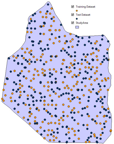
As an example consider the sample point population shown in Figure 2, which has been split into a training dataset (yellow points) and a test dataset (blue points).

Figure 2 – Split of a sample population into training and test datasets.
For the particular petrophysical variable we are modelling in this example, our knowledge of the geological setting would tell us that the predominance of a local variation is expected. Therefore the spatial proximity of points within the range of the expected local variation should be the main element considered when splitting the original input dataset into two subsets.
Magnitude of the Uncertainty
Now, let’s assume we have derived various models by using different algorithms and optimising the parameters which control the interpolation process, such as the search neighbourhood, power, and factors controlling smoothing and anistrotropy.

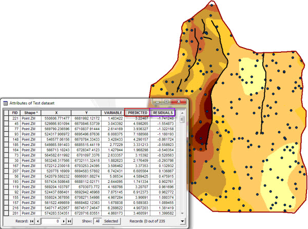
Figure 3 – Predicted values and residuals at the test dataset point locations
The first element we can consider to evaluate the quality of each prediction (model) is the magnitude of the residuals. It is easy to understand how the performance of our predictions can be directly correlated to the magnitude of the residuals, with the most reliable models showing the lowest residuals values.
The overall magnitude of the residuals can be estimated by a simple parameter called Root Mean Squared Error (RMSE) index. Although this parameter may be affected by the presence of bias in the residuals population, it has the great advantage of being easy and quick to derive. It can be used to obtain a first idea of the quality of the predictions, with lower values of RMSE indicating lower magnitude of errors.
As an example consider Table 1 which summarises the RMSE values for four deterministic models derived by using different local interpolator algorithms available in ArcGIS Spatial Analyst: Inverse Distance Weighted (IDW), Natural Neighbors (NN) and Spline (with and without barriers). The training dataset of Figure 2 was used to derive the models, while the test dataset was used to derive the residuals at the measured locations.
Note how the ‘Spline (with barriers)’ algorithm in this case provides the smallest RMSE, indicating that the overall values of the residuals are smaller for this model than for the others.

Table 1 – Model performance comparison matrix
Two additional indices can be used jointly to obtain additional information on the magnitude of the uncertainty (see Table 1). The Mean Absolute Error (MAE) measures the average absolute difference between observed and predicted values and is simply expressed by the mean of the absolute values of the residuals (e.g. not considering whether the prediction over or underestimates the observations). It provides a simple and quick estimation of the magnitude of the bias of the models and, as a consequence, better performing models are the ones with least prediction bias and, thus, smaller MAE.
It is very useful to evaluate the magnitude of the bias in our models in conjunction with the variance of absolute residuals. The Error Variance (EV) is a measurement of the precision (or lack thereof) in our predictions; a high value in the variance of our residuals indicates a smaller correlation between predictions and observations and, therefore, a poorer performing model. Ideally, therefore, we want to minimise the variance in the population of our residuals.
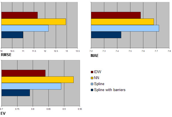
It is often useful to evaluate the MAE and the EV indices together, as large MAE and relatively large values of EV can be considered an indication of larger discrepancies between predictions and observations. Figure 4 below shows graphs of the magnitude of the three indices presented so far for each of the the four models.

Figure 4 – Comparison of uncertainty magnitude indices for four deterministic models
It can be seen how the ‘Spline with barriers’ model consistently provides the smallest residuals (RMSE and MAE) coupled with the smallest values in the variance of the residuals.
The comparison of these simple indices indicates that, for the example considered here, the ‘Spline with barriers’ algorithm is more capable of capturing the spatial characteristics of the petrophysical variable we are modelling than the others considered here.
To be Continued….
This is the second of a three-part blog on the subject of the estimation of uncertainty, if you missed it you should first read Part 1 of “How can I measure the quality of my predictions?”
In part 3 of “How can I measure the quality of my predictions?” I will discuss how the distribution of the residuals and the spatial component of the uncertainty can be brought within the analysis.
Posted by Paola Peroni, Senior Consultant, Exprodat.
Paola will be presenting elements of this methodology at the ESRI User Conference, Tue Jul 13th, 2010 (room 28 C), in San Diego.


