Investigating the Correlation Between Formation Pressure and Depth using ArcGIS
 Determining whether or not two or more continuous variables are correlated in space or time and quantifying the nature and the strength of this correlation is a type of data analysis which is common in many fields including physical geography, environmental studies and earth sciences. In geology, for instance, it’s been used to evaluate the relationship between stratigraphic horizons and the recent surface topography to provide insights on crustal movements caused by subsurface geological structures and faults1.
A simple way to investigate the degree of dependency of two continuous variables is to use an index called the Correlation Coefficient, which expresses in basic terms (a number between -1 and 1) the nature (negative, positive or no relation) and strength of the linear relationship between phenomena across space and time. In order to compute the Correlation Coefficient various statistical parameters (such as mean and standard deviation) are required.
As a means of testing the capability of ArcGIS Desktop to automate this computation for variables relevant in exploration of natural resources, I put together a model using Model Builder in ArcToolbox. The idea is to automate the sequence of steps to compute the statistics parameters within a chosen neighbourhood shape and size for any two continuous variables which are linearly correlated.
In the results discussed below you can see how easily such tasks can be automated using ArcGIS Desktop. The workflow can be applied to a variety of analysis and modelling tasks and is not, necessarily, confined to the world of oil and gas exploration.
A bit of more context, the data I used and the workflow I followed for my test.
My example represents a pretty common task for geoscientists, and deals with investigating the correlation between the values of the formation pressure (Variable 1) measured at some level within a known (or potential) reservoir and the depth to the top of the horizon (Variable 2) – ideally the contact between the reservoir and the seal. In my case I wanted to build a “proof-of-concept” test focusing on a relatively small scale, to have a feeling for whether ArcGIS could be used to carry out more regional-scale analysis to identify, for instance, areas of anomalies in pressure values.
In ideal conditions, such as having petrophysically homogeneous reservoir and seal with no faults, I would expect the reservoir formation pressure and depth to the top of the reservoir to be correlated. A deviation from this behaviour would indicate the presence of possible anomalies which could suggest, for instance, local permeability changes, lithological barriers or changes in the quality of the top seal.
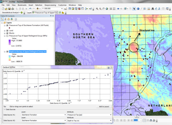
For my test I used a subset of data from the well-known Rotliegend gas play in the Dutch sector of the southern North Sea, therefore investigating only a small part of the gas system. The Rotliegend play comprises the prolific Westphalian source rocks for gas, the thick Slochteren sandstone reservoir, and a seal of Zechstein salt (Glennie & Provan,1990). Formation pressure and the modelled horizons for this play are in the public domain, and can be downloaded from the Netherlands Oil and Gas portal2. Note that there is an increase in the depth of the top of the Slochteren Formation from SE to NW, with structural lows determined by the fault system affecting this area (see Figure 1 below).
Figure 1 – Location of my test area. Note the structural lows indicating a sudden drop in the depth to top Slochteren Formation. Use of the General QQ Plot tool to explore the nature of the relationship between formation pressure and depth to the top of the geological horizon is shown on the left.
Because the Correlation Coefficient assumes linearity of the relationship among phenomena, the first task in my workflow is to check whether this is true for my two variables. To do this I extrapolated the pressure measured at various depths at my well locations up to the top of the Slochteren Formation reservoir. Not having access to the value of the pressure gradient for each well, I arbitrarily assumed that the vertical variation of the pressure is constant throughout my reservoir3. This assumption is obviously gross simplification, although it does not undermine the validity of the general approach.
I computed the depth to top Slochteren from the depth to its base and its thickness. From this grid I extracted top depth values at the well locations where I had measured pressure and used my assumed constant pressure gradient to extrapolate the pressure at the top of the reservoir. Following this approach I ended up with two point datasets.
I then used the ArcGIS Geostatistical Analyst General QQ Plot tool to investigate the nature of the relationship between my two variables. The plot is shown in Figure 1. Note that the plot indicates a fairly linear relationship between depth and pressure. In such a case I can use the Correlation Coefficient to represent a statistically reliable measure of the degree of dependency among my phenomena. Following the linearity check, I interpolated point values to generate a raster surface for the formation pressure at the top of the reservoir.
The model
At this point of my workflow I obtained the input datasets my model needed to compute the Correlation Coefficient.
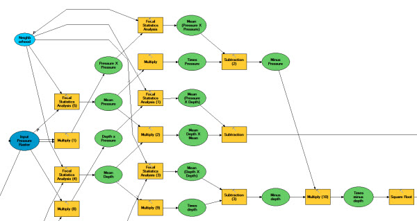
I had previously created a toolbox in ArcGIS called Pressure Analysis Tools containing two models (Figure 2A). The one called ‘Preprocessing’ simply prepares the data for the correlation analysis (which is needed in my case as the spatial extent and the cell sizes of my raster datasets are different). The actual correlation analysis is carried out by the one called ‘Calculate Correlation Coefficient’ (see an extract in Figure 2B).
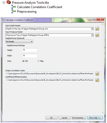
Figure 2A – ArcGIS custom toolbox.
Figure 2B – ArcGIS model.
As you can appreciate from Figure 2B, the model uses the concept of focal statistics to compute the statistical parameters needed to derive the correlation grid. Focal statistics computes various statistical parameters for a defined neighbourhood shape and size which is repeatedly “moved” throughout the study area. See the ArcGIS online help for further information about using focal statistics in ArcGIS.
The output of my analysis is the result of a moving-window computation of the statistical significance of the relationship between the depth and the pressure at the top of my reservoir. Given that the correlation is computed within each moving window, the use of a focal statistics approach has the advantage of being able to take into account local variations in the degree of dependency across the region of interest.
Results
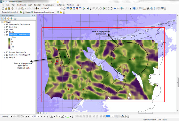
The result of the correlation analysis for my study area is shown in Figure 3.
Figure 3 – Correlation test between depth and pressure at the top of the Slochteren Formation.
As you can see the correlation map created show areas of high positive correlation (dark green) alternating with areas of high negative correlation (dark purple).
The positive correlation pattern is strong especially in the eastern part of my study area (area A in Figure 3), where my data indicates a transition between high and low pressure zones. It’s interesting to note that the area of the structural low highlighted in Figure 1 (area B in Figure 3) shows high positive correlation with the pressure, whose values increases sharply in line with the sudden deepening of the top of the reservoir.
Throughout my study region pressure and depth generally show a strong relationship, either positive or negative: anomalous areas in which there is no relationship between these two variables are limited (lightest areas). This suggests that depth to the reservoir is indeed one of the factors which control pressure values for this specific stratigraphic unit.
Clearly my analysis misses a number of other complex, key elements which the geoscientist may want to take into account (fault system, burial depth, fluid overpressure values, location of salt structures in the Zechstein sealing horizon, etc.), but hopefully you can see how GIS technology provides powerful tools to carry out and automate analysis workflows.
Posted by Paola Peroni, Senior Consultant, Exprodat.
- Lehne’ R. and Siroko F., (2005): “Quantification of recent movement potentials in Schleswig-Holstein (Germany) by GIS-based calculation of correlation coefficients” – International Journal of Earth Science (2005) 94: 1094-1102.
- The datasets I have used for this test are freely downloadable from the NLOG Oil and Gas data portal. Formation pressure values are available in a simple Excel spread sheet format, while depth to the base and the thickness of various horizons of interest for Oil and Gas exploration and production are available in grid format, ready to be used in ArcGIS.
- In my test I only used the pressure values for the water in the pores of the reservoir. Other fluids overpressure such as gas, oil, condensate or any mix of these was not considered.

